
CFD simulation of SUPERCHIMNEY (atmospheric reactor)
Abstract:
The idea of the Superchimney as an atmospheric reactor was introduced more than ten years ago by Michael Pesochinsky. Over that time the theory explaining how the Superchimney reactor works was introduced and small-scale testing was conducted. Despite successful implementations, critics of the concept maintained their main objection to the proposed model: that the reactor will not work because of adiabatic cooling happening inside the chimney. The following study created a mathematical model which was implemented using a CFD simulation method. The results decisively demonstrate that the Superchimney works and no substantial adiabatic cooling can take place inside the chimney. Moreover, if such a Superchimney were ever built it will work and produce incredible airflows.
1- INTRODUCTION
The physical principle underlying the Superchimney is simple: Hot air rises above cold air because hot air is less dense. Therefore, it is lighter than cold air. In atmosphere, masses of warmer air are constantly moving up while cooler air goes down. The chimney facilitates that upwards motion of air by preventing the mixing of air with the colder surroundings. This stops adiabatic cooling from happening to the parcels of air as the air is rising.
Normally, when hot air freely rises in atmosphere it expands as it gets higher and pushes the surrounding air. That causes the surrounding air to heat up and the rising air to cool. That process continues until equilibrium is reached. At that point air stops its ascending.
Unlike a freely rising parcel of air, the air in the chimney is restricted in its horizontal expansion and thus it is NOT free rising. When air rises in the chimney it also expands, but only in the upper direction. It compresses the layer of air above it, heats it up and loses its own heat. At the same time the air below does the same thing. Layers of air are being pushed and push themselves all the way to the exit of the chimney. This results in maintaining the same amount of heat in every layer of air. This is how the chimney works.
Notice that this explanation is different from the conventional explanation, which refers to air draft caused by heating air inside the chimney. Unlike the conventional explanation, the proposed mechanism states that air will flow inside of the chimney as long as the air below is warmer than the air above. There is no need for additional heat (like fire) to make the air move.
Now, let us consider our atmosphere. As we climb up, the temperature drops 10° C (roughly 20° F) every 1000 meters (roughly 2/3 of a mile). Let us just assume we can build a chimney 5 kilometers (3 miles) high. Let us call it a Superchimney. The air at the base of this Superchimney will be roughly 50°C (100°F) warmer than at its top.
According to the Superchimney proponents air inside such a chimney will be moving up at incredible speeds. According to the opponents the air inside the chimney will act just as the air outside and will be cooling down, thus reaching equilibrium and not moving up.
These studies were set up to answer that question using computational fluid dynamics (CFD) to simulate what will happen in the chimney. As well as to determine whether the air will move without any additional heat sources such as green houses, fire etc.
2- Methodology: COMPUTATIONAL FLUID DYNAMICS
The simulation was conducted using Computational Fluid Dynamics software, namely ANSYS FLUENT 19. As the work was conducted many technical issues came up. There were limitations on the computer power available. Also, there was lack of any other research within this field. As result certain compromises were made:
1. Creating a simulation of our atmosphere proved to be impossible. The task is too complex and involves many factors which cannot be considered by the CFD software alone. Instead of creating a simulation of the atmosphere we created boundary conditions which replicated our atmosphere inside the domain.
2. The size of the domain was limited to the bare minimum because of computational constraints
3. While the results definitively answer the question of whether or not the Superchimney will work, they cannot be used for engineering calculations because of the multiple assumptions designed to simplify the solution. The true speeds of air inside the chimney can be determined only when a pilot chimney is built and physical properties are measured (air speed temperature, pressure etc). Additionally, the studied design, which is a mere cylinder, is not the best from an air dynamic point of view. It can be substantially improved to increase the efficiency.
Once all geometric, meshing and physical data were introduced into the model it was uploaded to the CFD software in order to find a solution. All CFD software contains algorithms that numerically solve the partial differential equations describing the movement of any fluid, the Navier-Stokes equation.
![]()
Figure 1 : Navier-Stokes equation
This version of the equation is called the Averaged Navier Stokes equations (RANS). It addresses turbulent flow in a much more practical way in order to achieve a faster and simpler resolution.
Figure 2: Reynold’s Averaged (RANS) Navier Stokes Equations
Solving that version of the Navier–Stokes equation produced the simulation results described below.
3- Simulation set up, domain, boundary conditions
Numerous research papers cover the extreme complexity of the different layers in which atmosphere is divided as well as the multiple phenomena that take place in it.
In addition to rising currents of hot air, lowering of the upper cold air and the effect of the wind, there are several other phenomena which are too complex to address through simulation. These phenomena include mesoscale and synoptic scale structures, evolution of water vapor, influence of radiation, earth´s Coriolis acceleration, localized breezes and other localized phenomena, etc.
In order to accurately capture all these effects, a more evolved tool than CFD is required. This is due to the phenomenal computing power required to analyze them in a 3d discretized domain. All these phenomena have been excluded from the present analysis, which intends only to demonstrate the mechanism of air rising in a giant chimney and to prove that the adiabatic cooling phenomenon is impossible inside a chimney. The below factors were considered and used in our calculation:
· Compressible behavior of air. - The behavior of air adapts to the height or the pressure created inside the Superchimney.
· Solar gain on the ground due to sun irradiation. - This is responsible for the hotter initial layers of air on the ground.
· Zero pressure on top of the domain in order to simulate the end of the known atmosphere
· Pressure gradient to the ground. - This accounts for the static pressure present at each height level as we move away from the ground towards upper heights.
· Temperature gradient to the ground. - This accounts for the lower temperature that air shows as height increases.
· The walls of the Superchimney do not conduct heat. - This is so that no heat exchange takes place between the interior air and the colder exterior air.
DOMAIN
The domain considered in the simulation consists of a square domain in which the Superchimney is installed and has enough space around it to allow the buildup of air currents typical for this kind of obstacle.
The domain has a height of 10km, allowing the installation of a 5km high Superchimney while still having enough space for the air currents above the chimney´s exit to build properly.
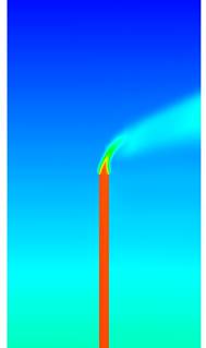
The width and depth of the domain are equal and extend 250m, forming a square in the base. This relatively small size was chosen in order to minimize the computational load as computing resources were limited to just one server. However, this size is sufficient to demonstrate the mechanisms of air rising inside the chimney. The Superchimney is 10m wide and located in the middle of the domain It is elevated 250m from the ground (so it can absorb air) and reaches a height of 5000m at its exit.
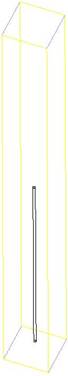
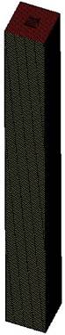
Figure 3: Overall view of the geometry and hexahedral mesh of the domain
TURBULENCE MODELLING
A 2-equation turbulence model was used in order to achieve a realistic influence of turbulence and correctly capture the boundary layer region (which however small in size can have a significant influence on the air currents generated).
The chosen turbulence model was K-w SST, which automatically switches between wall functions and boundary layer calculation depending on the dimensional distance to the wall (Y+). The main advantage of this model is that it allows use of same first cell size all across the domain without worrying about correctly capturing the Y+ value. This feature makes the model computationally more expensive than the other 1 equation models such as Spalart-Allmaras.
BOUNDARY CONDITIONS
The boundary conditions required to reproduce the working Superchimney are extremely complicated due to the complexity of all involved phenomena. However, as all meso- and synoptic scales have not been included, the boundary conditions are simplified, resulting in following setup:
Sides and wind:
On one side a “pressure inlet” condition was used in which the speed, temperature and main turbulence parameters of incoming air are specified. On the opposite side a “pressure outlet” condition was applied to allow for the air to leave the domain.
However, these boundary conditions may not be used with their default configuration because they are defined as constant all across the boundary. Some additional variables need to be introduced in order to account for the thermal and pressure stratifications present in real atmosphere.
On both boundaries (left and right limits of the domain) the temperature was linearly changed from top to bottom of the boundary, starting at -70ºC at the top and finishing at +40ºC on the bottom.
The same strategy was used for the pressure on the right side (0 atm at the top and 1 atm at the bottom). On the left side the same pressure and temperature distributions are used in order to account for the atmospheric gradient for those variables.
In order to guarantee a constant flow of air from the left to the right sides of the domain, a 20 Pa increase was applied on the pressure distribution. This was done in order to generate some momentum in the air and not let the numeric residuals influence the stability of the simulations.
Top:
On top of the domain a “pressure outlet” condition has been applied (0 atm) to allow for air entering or exiting the domain as the simulation sees fit. This boundary condition was used instead of installing a solid wall on top of the domain, as that would influence the pressure distribution of the whole domain as the simulation advances.
Bottom:
A simple “solid wall” condition has been applied to account for the ground effect and the effect of the sun, defining the temperature of the ground as +40ºC to account for sun irradiation and avoid localized temperature variations on the ground.
Superchimney:
The walls of the chimney have been defined as a solid wall with no heat conductivity. The main purpose of this is to prevent thermal losses in the chimney and obtain the maximum theoretical performance associated with the current design.
Initialization:
On top of defining temperature and pressure gradients on the sides of the domain, the simulation must be correctly initialized in order to allow the buildup of the desired flow within the Superchimney.
Due to the huge length of the chimney, it is suspected that it will take quite a long time for an air draft to have enough energy to create a stream along the whole chimney. This means that some kind of kick-start will be required. This is a common practice when starting up hydraulic nets, pumps and other devices that require priming.
For this reason, the initial state from which the simulation started consisted of a lateral air current with the corresponding thermal and pressure stratifications (swiping from left to right of the domain) and the interior of the chimney full of air at the maximum temperature (+40ºC). This was done to help the chimney create the initial updraft that, later on, will be maintained by the temperature differences in the upper and lower atmospheres.
In order to obtain this initial flow field, a transient simulation was launched. In this simulation the interior of the Chimney was full of hot air (+40ºC) in order for it to start rising as soon as the simulation starts. As time in the simulation passes, pressure, density and other variables adjust to realistic distributions inside the chimney. This is done in a way that a user can never describe as an initial solution for a stationary simulation.
MESH
In order to obtain the best possible convergence of the simulation, a structured hexahedra mesh was generated in the domain.
The generated mesh consists of 250.000 hexahedra and, due to the simple geometry used (square domain with a round chimney in the center), a very uniform topology was used, keeping the skewness of all cells under 0.1 (considered excellent mesh quality).
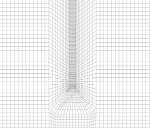
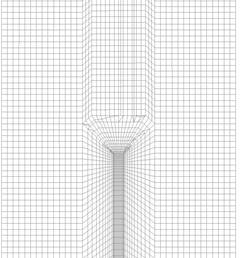
Figure 4 : Detail of the hexahedral mesh at the entrance (left) and exit (right) of the chimney. Lateral view
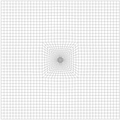
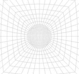
Figure 5 : Detail of the hexahedral mesh through the chimney. Top view
Results
4- STATIONARY SIMULATION
As the first step, a stationary simulation was set up and run in order to know the chimney works once it reaches its equilibrium state (when it is working outside of its initial phenomena during the first minutes). The physics and boundary conditions used are the ones already detailed in the previous chapter, except that the simulation is launched without keeping track of time.
Once the simulation converges, it reaches a solution and we can then observe the pressure, speed and temperature distributions throughout the whole domain. The following images show the distribution of these variables in different regions of the domain.
The most relevant parameter, due to its importance in defining the airflow, is the pressure distribution.
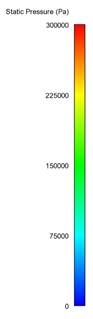
Figure 5 : Pressure field through the middle plane of the domain
On top of the pressure gradient, between the top and bottom of the domain, the most relevant feature detected in the pressure distribution is the difference between pressure inside and outside the chimney.
Pressure lowers as we move towards the top, but the change rate is different inside the chimney, where it gets slightly lowered more quickly on its way up. This difference in pressure variation is associated with the lack of adiabatic cooling inside the chimney, which accelerates the pressure reduction as we increase in height.
As a secondary phenomenon, the pressure is also modified at the inlet and outlet regions of the chimney. This pressure distribution is the consequence of an air stream flowing by the inlet and outlet of the chimney, which were simulated as simple cylindrical tubes.
These local pressure distributions also play a role in the definitive mass flow reached by the chimney. This is because of their strategic location right at the entrance and exit of the chimney. In other words, the geometry of these regions could be designed so that the pressure distribution helps the flow inside the chimney and increases flowrate; however, this optimization has not been explored in the current analysis as it is outside the current work scope.
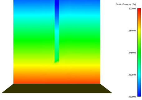
Figure 7 : Pressure distribution through middle plane at the chimney inlet region
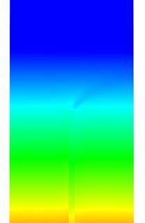
Figure 8 : Pressure distribution through middle plane at the chimney outlet region
If we measure the static pressure inside the chimney on its center line, we will obtain the evolution of pressure with height. This turns out to be quite linear when evaluated macroscopically.
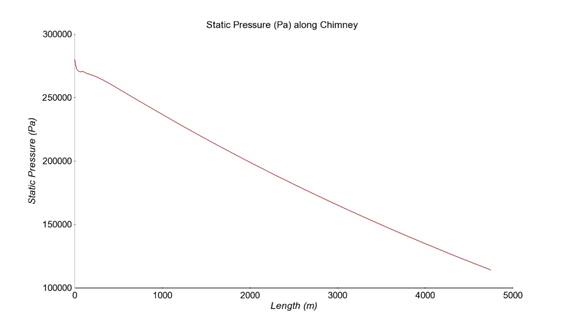
Figure 9 : Pressure distribution long chimney´s centerline
The distribution of the rest of the parameters is a direct consequence of the pressure distribution.
The following images show the velocity distribution in the whole domain along with a close-up view of the entrance and exit of the chimney.
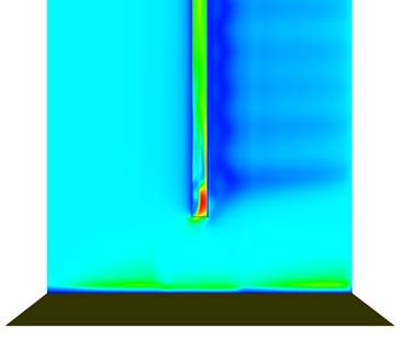
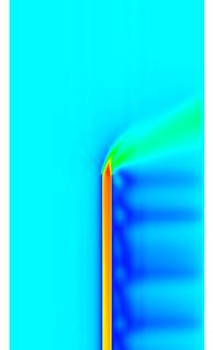
Figure 10 : Velocity distribution through middle plane at the chimney inlet (left) and outlet (right) regions
![]()
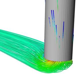
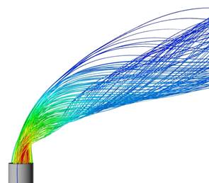
Figure 11 : Velocity flow tracks at the chimney inlet (left) and outlet (right) regions
As was expected, the exact velocity distribution of air as it enters or exits the chimney is conditioned by the geometry it has to flow through. The design used in those regions, a simple cylindrical shape, does not help increase the flowrate in any way.
Some improvement is expected when a more detailed design of these regions is used. They will reduce the energy losses, thereby increasing the flowrate under the same flow conditions.
The following graph shows the air speed value along the chimney´s centerline. In spite of having some local secondary flows at the inlet and outlet regions, the length of the chimney (4.750m) makes it quite insightful.
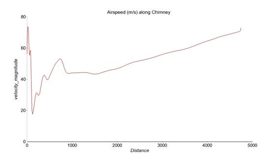
Figure 12 : Airspeed along chimney´s centerline
The temperature evolution responds only to the change caused by the pressure changes because the chimney walls were defined as 0 heat conductivity. Therefore, once the air enters the chimney its temperature remains unchanged unless the pressure evolution causes otherwise.
The following images show the temperature distribution in the whole domain along with a close-up view of the entrance and exit of the chimney.
![]()
![]()
Figure 13 : Temperature distribution throughout the domain (middle plane)
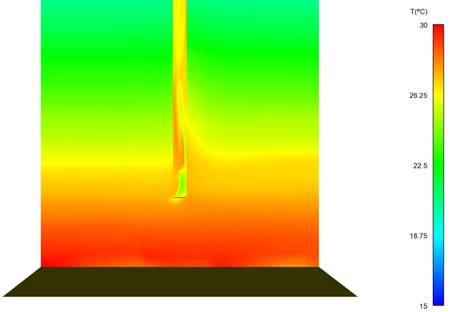
Figure 14 : Temperature distribution through middle plane at the chimney inlet region
![]()
Figure 15 : Temperature distribution through middle plane at the chimney outlet region
The following graph shows the temperature distribution along the chimney´s centerline. Entrance and exit regions aside, the overall temperature variation is also quite gradual as it gains height.
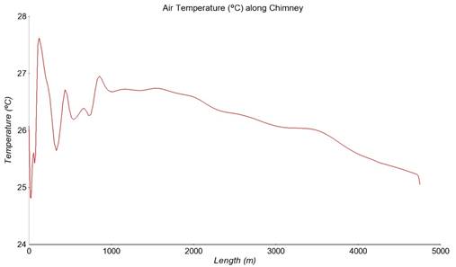
Figure 16 : Temperature along chimney´s centerline
Summarizing the results, it can be concluded that a 4.750 m chimney connecting the lower and upper atmosphere (5 km height) does create an upward draft powered by the lack of adiabatic cooling inside. The speed reached at the exit of the chimney is approximately 80 m/s and its temperature has lowered around 2 ºC which is negligible. This can be attributed to the drop of static pressure and demonstrates that adiabatic cooling did not happen.
However, it must be kept in mind that in order to reach this state an initial priming of the chimney is necessary. In this case we started with a chimney full of hot air (air at ground temperature, 40ºC). A solution that begins with an empty chimney has not been achieved.
This simulation does not deliver any information regarding how long it takes the chimney to reach this state. In order to obtain more information regarding its dynamic behavior, a transient simulation was launched with the same model.
5- TRANSIENT SIMULATION
In this kind of analysis, a simulation is carried out which considers time and provides a solution at every timestep. The length of the timestep, and therefore the degree of time advance as the simulation runs, depends on many factors. The cell size is one of the most restrictive factors. Considering how this case has been modelled and meshed, a 0,001 timestep was eventually used, simulating a total of 169s. It is also critical to remember that the initial state (situation at 0 s) assumes a primed chimney (full of hot air).
Flow field details aside, the time evolution of some main parameters (such as air speed or temperature along the chimney) give valuable information. They show how quickly (or slowly) the initial hot air leaves the chimney and that it starts working by itself, powered by adiabatic expansion.
The following graph shows the air speed inside the chimney at the outlet as time passes.
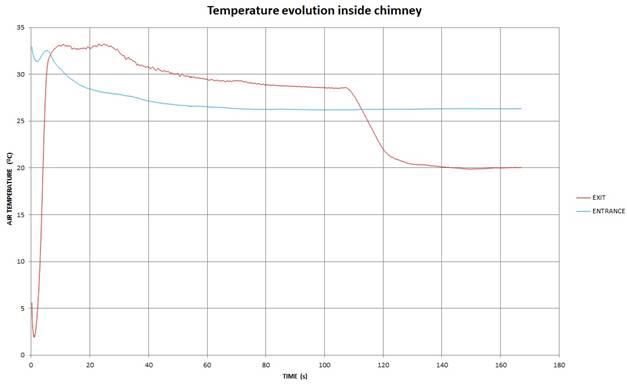
Figure 17 : Temperature evolution with time at chimney entrance and exit
The most relevant feature shown in this graph is the time it takes the chimney to empty the initial hot air used to prime it. After approximately 110s the hot air inside the chimney runs out. This shows that the reason the chimney continues to work is NOT because of the artificially placed pocket of hot air. From 110s on the temperature of air inside the chimney stays roughly the same. The temperature difference achieved between the entrance and exit of the chimney, once it is working by itself, is approximately 6ºC. This can be explained by some adiabatic cooling at the very exit of the chimney and air expansion due to the drop of static pressure inside the chimney.
The next graph shows the air speed at the chimney exit as time goes by.
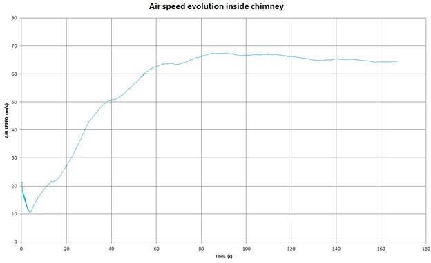
Figure 18 : Air Speed evolution with time at chimney entrance and exit
It can be clearly seen that air inside the chimney accelerates as time goes by. This implies that the buoyancy of the initial hot air is quickly surpassed by the power of the absence of adiabatic cooling. This gradually increases airspeed as the initial buoyancy dissipates and reaches a maximum when this initial hot air runs out.
Care must be taken when comparing the data from the stationary and transient simulations, especially regarding the airspeed values. In the stationary simulation the data was read on the centerline of the chimney, obtaining punctual values. However, in the transient simulations an average over the whole exit area was performed, obtaining an average value which is lower. This is because it includes the lower speed values as we get closer to the wall of the chimney.
Considering all these parameters, it can be concluded that a chimney primed with air at ground temperature would complete its start-up cycle after approximately 2 minutes. Ffrom there it sustains itself, generating a 65 m/s air current or higher.
We created 4 video simulations to help visualize the process of a chimney starting with warm air inside and then running with ambient air. The simulations show the temperature and air speed at the entrance and exit of the chimney.
Links to Youtube:
Temperature at the superchimney entry --- https://youtu.be/JTDr6AN83coTemperature at the superchimney exit --- https://youtu.be/WeO-qMcvQSU
Air velocity at the superchimney entry -- https://youtu.be/N1XtPmwYtPE
Air velocity at the superchimney exit --https://youtu.be/8SMjy3jTxH8
Data files for CFD are available upon request.
6- CONCLUSION
The idea of the Superchimney was suggested for the purposes of energy generation, water irrigation and, most importantly, to fight global warming. The calculations for these processes were developed and can be reviewed on the website superchimney.org. The present study developed the mathematical model for the SuperChimney based on CFD methods. It proved that the Superchimney will act as a meteorological reactor which can produce tremendous airflows. We are now one step closer to achieving our stated goals.
 |